Numerical methods
Introduction
Suppose you are asked to solve this equation
$$ x^{4} - 3x^{3} - x^{2} + \frac{2}{\sqrt{x}} = 0 $$
It's not immediately obvious how to solve it using the algebra you've been taught.
Fortunately there are numerical methods that allow you to quickly find approximate (and accurate) solutions to equations.
In fact, you can find that the solutions to the above equation are approximately $x=0.86786, 3.273944$ in less than a minute with a little bit of differentiation and rearranging.
The main difference between analytical methods (the algebra you've been taught so far) and numerical methods is that of error. Algebraic solutions always yield exact answers. You can be sure without a shadow of a doubt that they're the absolute correct answers.
Numerical methods yield approximate solutions, that, while highly accurate, are ever so slightly 'wrong'.
However, in real-life solutions like in engineering, where numerical methods are used extensively, it does not really matter if your answer is not absolutely correct to the 20th decimal place. It is often sufficient to find an answer that is correct to, say, three or four decimal places depending on the problem at hand.
Most numerical methods are iterative, meaning you start off with some initial conditions, and run the same steps over and over again. You can go for as many iterations as you want - more iterations usually gives you a more accurate answer.
Finding roots
In FP1 you will learn three methods for solving equations. These are the bisection method, linear interpolation, and the Newton-Raphson method.
In the first two methods you will need to understand Bolzano's theorem and how it relates to solving equations.
Firstly, the intermediate value theorem (IVT) states that if a function $f(x)$ is continuous across some interval $a \le x \le b$, then $f(x)$ may be equal to any value between $f(a)$ and $f(b)$.
A special version of IVT is Bolzano's theorem, which states that if a function $f(x)$ is continuous across some interval $a \le x \le b$, and $f(a)$ and $f(b)$ are on opposite sides of the $x$-axis (one is positive and the other negative), then a root of $f(x)$ lies in between $a$ and $b$.
Here's a diagram that shows what this means
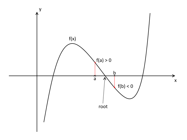
This is important because it helps us to make an accurate guess for where a root of an equation might lie. If we know that for some function $f(2) = -1$ and $f(2.5) = 2$, then we know that a root lies somewhere between $x=2$ and $x=2.5$.
The bisection method
The bisection method for solving an equation involves finding an initial interval where a root lies, using Bolzano's theorem, and then in each successive step halving the interval to get a smaller and smaller interval and eventually reach an interval whose midpoint will be the approximate solution.
These are the steps
- Find a suitable interval $[a,b]$ such that $f(a) \gt 0$ and $f(b) \lt 0$ or vice versa.
- Compute the midpoint $m$ of the interval, $m= \frac{a+b}{2}$.
- Compute $f(m)$.
- If the answer is sufficiently accurate stop iterating and return $m$ as the approximate solution.
- Check whether $f(m)$ is positive or negative.
- Replace $a$ or $b$ with $m$ so that the root is still within the new interval.
- Repeat from step 2.
In the exam they will usually ask to give your answer to a certain degree of accuracy, e.g. one decimal place. Once your answer is that accurate, you can stop the method and you will have the required answer.
As you keep halving your interval, you will find that each new $m$ gets more and more decimal places. Once the difference between your current $m$ and the last $m$ is less than the number of decimal places they have asked you for, you can stop the method and the current $m$ is the answer.
Example
Q) Find an approximate solution to $x^{5} - x^{4} + 1 = 0$ using the Bisection method correct to one decimal place, given that the root is in the interval $[-1,-0.5]$.
A) Indeed $f(-1)=-1 \lt 0$ and $f(-0.5)=0.90625 \gt 0$.
The first midpoint $m_{1}$ is $\frac{-1-0.5}{2} = -0.75$.
$f(-0.75) = 0.446\ldots \gt 0$, so the new interval is $[-1,-0.75]$.
The second midpoint $m_{2}$ is $\frac{-1-0.75}{2} = -0.875$.
$f(-0.875) = -0.099\ldots \lt 0$, so the new interval is $[-0.875,-0.75]$.
The third midpoint $m_{3}$ is $\frac{-0.875-0.75}{2} = -0.8125$. This is less than one decimal place different from $m_{2}$, so our answer correct to one decimal place is $-0.8$.
Linear interpolation
Linear interpolation is an extension to the bisection method. Starting with an interval $[a,b]$ where a root lies you make a straight line between the points $f(a)$ and $f(b)$. Using similar triangles you can find the root of this straight line, which we call $\alpha$. $\alpha$ is then that iteration's approximation of the solution, and a candidate for a new boundary point to replace $a$ or $b$, depending on whether $f(\alpha)$ is positive or negative.
Here's a diagram to illustrate it
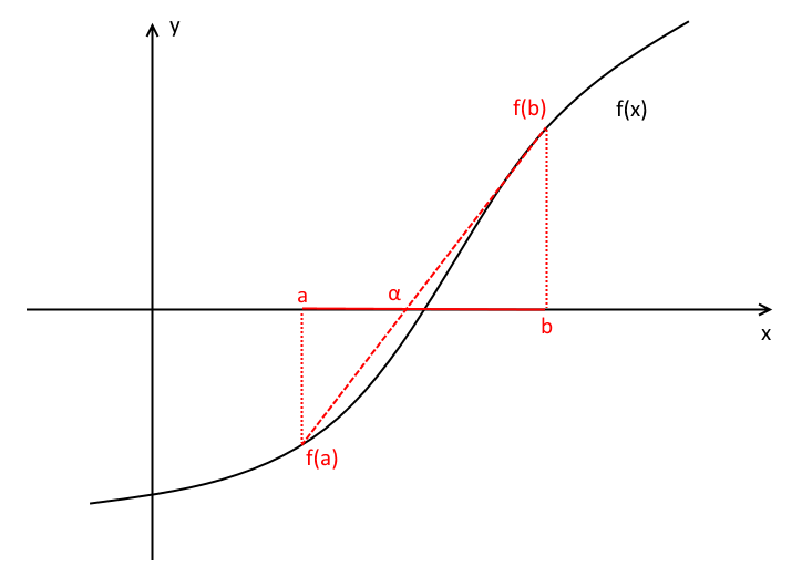
At each iteration to find $\alpha$ you need to use similar triangles and solve
$$\frac{\alpha-a}{b-\alpha} = \left|\frac{f(a)}{f(b)}\right|$$
Rearranging and putting the $\alpha$ terms on one side
$$ \begin{align} \alpha-a &= \left|\frac{f(a)}{f(b)}\right|(b-\alpha) \\ \alpha\left(1+\left|\frac{f(a)}{f(b)}\right|\right) &= a + \left|\frac{f(a)}{f(b)}\right|b \\ \alpha &= \frac{a + \left|\frac{f(a)}{f(b)}\right|b}{1+\left|\frac{f(a)}{f(b)}\right|} \\ &= \frac{a |f(b)| + b |f(a)|}{|f(b)| + |f(a)|} \end{align} $$
And we can use this directly at each iteration in lieu of solving for $\alpha$ over and over again.
These are the steps
- Find a suitable interval $[a,b]$ such that $f(a) \gt 0$ and $f(b) \lt 0$ or vice versa.
- Form a straight line between $f(a)$ and $f(b)$.
- Compute $\alpha$, the point where this straight line crosses the $x$-axis, using similar triangles.
- Compute $f(\alpha)$.
- If the answer is sufficiently accurate stop iterating and return $\alpha$ as the approximate solution.
- Check whether $f(\alpha)$ is positive or negative.
- Replace $a$ or $b$ with $\alpha$ so that the root is still within the new interval.
- Repeat from step 2.
Example
Q) Find an approximate solution to $x^{3} - \sin x = 0$ using linear interpolation correct to one decimal place, given that a root lies in the interval $[0.5,1]$. Give your answer in radians.
A) Indeed $f(0.5) = -0.354\ldots \lt 0$ and $f(1)=0.158\ldots \gt 0$.
Using our formula defined above, we find that $\alpha_{1} = \frac{0.5\times 0.1585+1\times 0.3544}{0.1585+0.3544} = 0.845$.
$f(\alpha_{1}) = -0.144\ldots \lt 0$ so the new interval is $[0.845,1]$.
On the second step we find that $\alpha_{2} = \frac{0.845\times 0.1585+1\times 0.1446}{0.1585+0.1446} = 0.9189$.
$f(\alpha_{2}) = -0.018\ldots \lt 0$ so the new interval is $[0.9189,1]$.
On the third step we find that $\alpha_{3} = \frac{0.9189\times 0.1585+1\times 0.0189}{0.1585+0.0189} = 0.9275$.
This is less than one decimal place different to $\alpha_{2}$ so our answer correct to one decimal place is $0.9^{c}$.
The Newton-Raphson method
The Newton-Raphson method is a much faster way of finding roots of equations than the other two methods, and less time-consuming to carry out.
Instead of finding a boundary to look in, you start off with an initial guess, $a_{0}$ that you think is sufficiently close to the actual root $\alpha$. You also need to find the first derivative of the function $f$ you're asked to solve.
Then you find each successive iteration by using the following formula
$$a_{n+1} = a_{n} - \frac{f(a_{n})}{f'(a_{n})}$$
Let $f(x)$ be a differentiable function, and $x_{n}$ be an approximation to a root of $f$.
Then the tangent line of $f$ at $x=x_{n}$ is
$$y-f(x_{n})=f'(x_{n})(x-x_{n})$$
Then find where this line crosses the $x$-axis to obtain the next approximation to the root, $x_{n+1}$. Set $y=0$ and $x=x_{n+1}$
$$-f(x_{n})=f'(x_{n})(x_{n+1}-x_{n})$$
Solve for $x_{n+1}$
$$x_{n+1} = x_{n} - \frac{f(x_{n})}{f'(x_{n})}$$
Example
Q) Find an approximate solution to $x^{2} - 2 = 0$ by using four iterations of the Newton-Raphson method. Use $a_{0}=1$ as an initial estimate, and give your answer to three decimal places.
A) Firstly, we see that $f'(x) = 2x$.
So our formula for each successive estimate is
$$a_{n+1} = a_{n} - \frac{a_{n}^{2} - 2}{2a_{n}}$$
Carrying out the iterations
$$ \begin{align} a_{1} &= a_{0} - \frac{a_{0}^{2} - 2}{2a_{0}} = 1.5 \\ a_{2} &= a_{1} - \frac{a_{1}^{2} - 2}{2a_{1}} = 1.41666\ldots \\ a_{3} &= a_{2} - \frac{a_{2}^{2} - 2}{2a_{2}} = 1.41415\ldots \\ a_{4} &= a_{3} - \frac{a_{3}^{2} - 2}{2a_{3}} = 1.41421\ldots \end{align} $$
And we are done. The approximate solution is $a_{4}=1.414$ (3.d.p.).
Note that an exact solution to $f(x)$ is $\sqrt{2} \approx 1.41421$, so this method quickly came close to the answer.
You are probably thinking why bother with the other two methods if Newton-Raphson is so good? Well Newton-Raphson sometimes fails to find a solution, depending on the gradient of $f$ around the iteration points. Exactly why this is the case is beyond the scope of FP1, but I thought you might like to know.